Algorithms
All algorithms share one loop; they differ only in the frontier (which
discovered node is expanded next) and the evaluation function
priority = g_coeff·g(n) + h_coeff·h(n). Select one with algorithm= and, for
the priority-based ones, a heuristic=.
Uninformed search
These ignore where the goal is; they differ only in the order they pull nodes from the frontier.
algorithm |
Frontier | Idea | Complete | Optimal | Memory |
|---|---|---|---|---|---|
bfs |
FIFO queue | expand by depth | yes | unit costs only | high |
dfs |
LIFO stack | dive deep first | finite graphs | no | low |
ucs / dijkstra |
min-heap | expand by g(n) |
yes | yes | high |
dls |
LIFO + limit | DFS cut at depth_limit |
within the limit | no | low |
iddfs |
repeated DLS | grow the limit each round | yes | unit costs only | low |
bidirectional |
two FIFO queues | frontiers meet in the middle | yes (symmetric) | unit costs | medium |
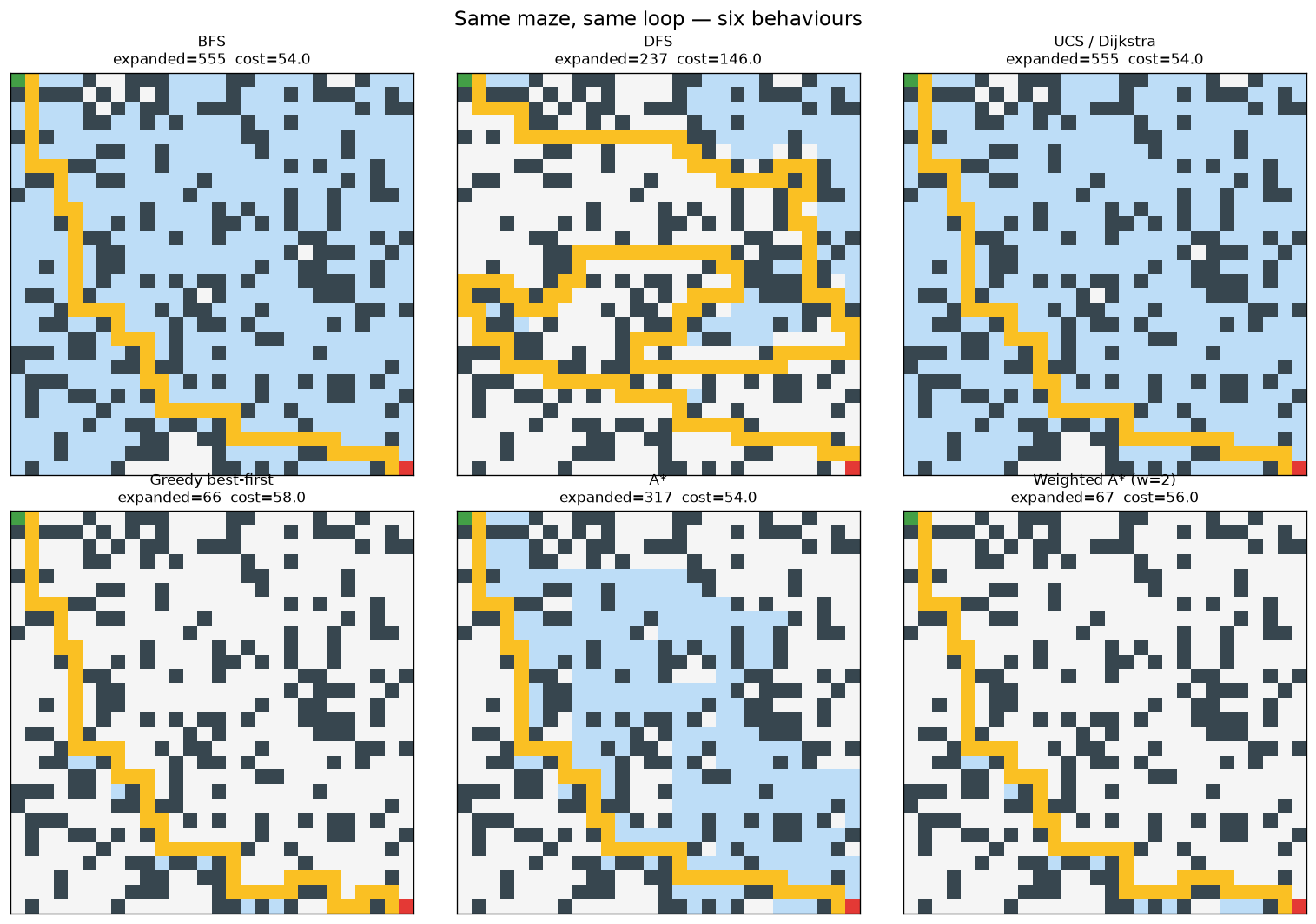
BFS vs DFS vs UCS. On a unit-cost grid BFS and UCS expand the same nodes and return the same optimal path; DFS finds a path quickly but it is usually far from shortest (in the figure above, cost 146 vs the optimum 54).
Iterative deepening (iddfs, ida_star) re-expands shallow nodes every
round, trading time for DFS-level memory — ideal when the graph is huge or
infinite and you cannot store an open list.
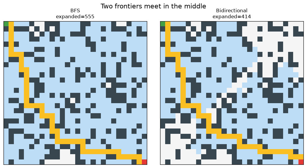
Bidirectional search grows a frontier from both the start and the goal and stops when they touch, exploring far fewer nodes:
Informed search
These use a heuristic h(n) estimating the remaining cost.
algorithm |
Priority | Complete | Optimal |
|---|---|---|---|
greedy |
h(n) |
no | no |
astar |
g(n) + h(n) |
yes | yes (admissible h) |
weighted_astar |
g(n) + w·h(n) |
yes | within w× optimal |
ida_star |
iterative deepening on g + h |
yes | yes (admissible h) |
beam |
best beam_width by h per level |
no | no |
Greedy rushes toward the goal by h alone — fewest expansions, but it can
commit to a costly route. A* balances cost-so-far and estimate, returning
the optimal path while expanding far less than UCS. Weighted A* inflates the
heuristic (weight=w>1) to go faster at the price of a bounded sub-optimality.
Beam keeps only the beam_width most promising nodes per level — tiny,
bounded memory, no guarantees.
Beyond the frontier: negative weights
Every algorithm above is a frontier traversal, and the optimal ones
(UCS/Dijkstra, A*) assume non-negative edge costs. When a weight can be
negative, use the relaxation/DP algorithms instead — bellman_ford (single
source, detects negative cycles) and floyd_warshall (all pairs). They are not
selected via algorithm=; they are their own functions. See
Shortest paths.
Parameters
| Parameter | Applies to | Meaning |
|---|---|---|
heuristic |
priority-based algorithms | a built-in name ("zero", "manhattan", "euclidean", "octile") or a custom callable h(node, goal) -> float (any domain) |
weight |
weighted_astar |
the w multiplier on h (default 2.0) |
beam_width |
beam |
frontier cap per level |
depth_limit |
dls (required), iddfs (cap) |
maximum search depth |
max_nodes |
all | expansion budget; stops early with stop_reason="node_limit" |
record |
all | keep the per-step trace (needed for visualization) |
diagonal |
search_grid |
8-connectivity (use with octile) |
Completeness & optimality at a glance
- Complete (always finds a solution if one exists): BFS, UCS, IDDFS, A*, Weighted A*, IDA*, bidirectional. Not complete on infinite graphs: DFS, Greedy, beam.
- Optimal (returns a least-cost path): UCS/Dijkstra always; BFS and
bidirectional on unit costs; A* and IDA* with an admissible heuristic;
Weighted A* within a factor
w. Not optimal: DFS, Greedy, beam.
Use viz.compare to see these trade-offs on your own
problem — the work-vs-quality bars make the difference obvious.