Visualization

graphfinder.viz turns a SearchResult into figures and animations with matplotlib. Every helper takes the result of a search run with record=True (needed for the per-step trace) and returns a matplotlib object you can further style or save.

pip install "graphfinder[viz]"   # matplotlib (+ pillow for GIFs, networkx for layouts)

All functions import matplotlib lazily, so importing the package stays cheap.

animate_grid — watch the search explore

The flagship. Replays each expanded cell, then draws the path.

r = gf.search(maze, algorithm="astar", record=True)
anim = gf.viz.animate_grid(maze, r, interval=40)
anim.save("astar.gif", writer="pillow", fps=25)     # or HTML(anim.to_jshtml()) in a notebook

Same maze, two strategies: A* (left) drives toward the goal; BFS (right) floods outward in rings. The contrast is the whole point of informed search.

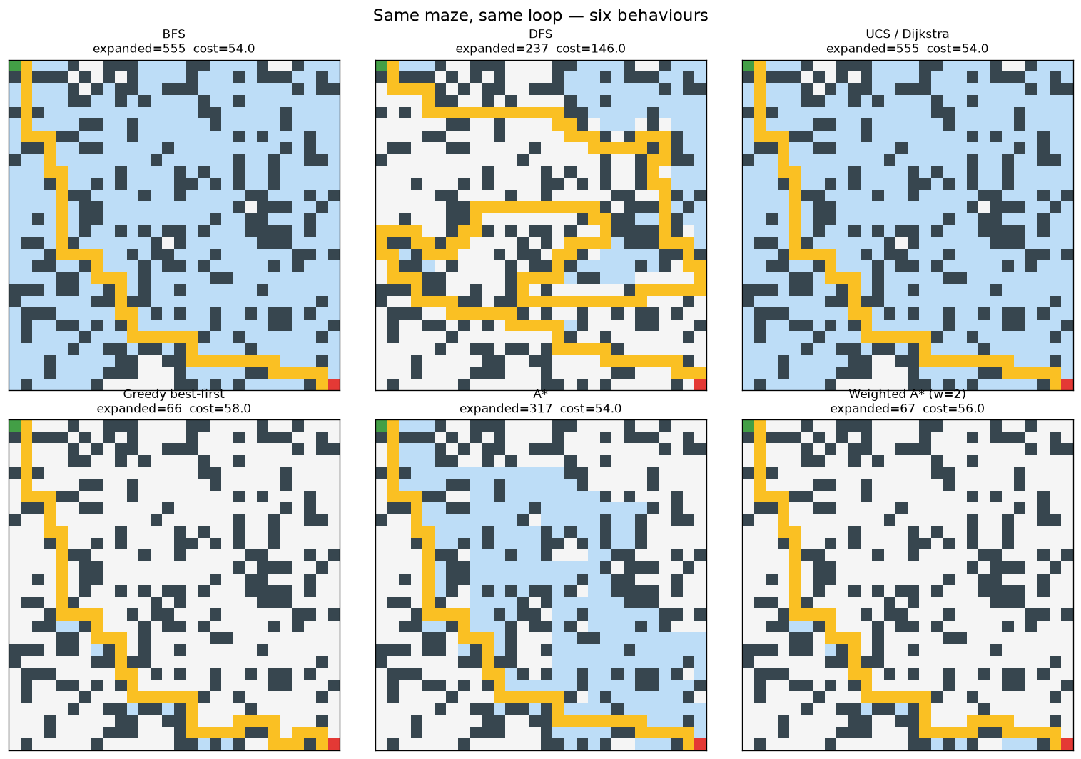
plot_grid — static snapshot

A single frame: walls, every expanded cell shaded, the path on top.

gf.viz.plot_grid(maze, r)

Stack several to compare algorithms at a glance:

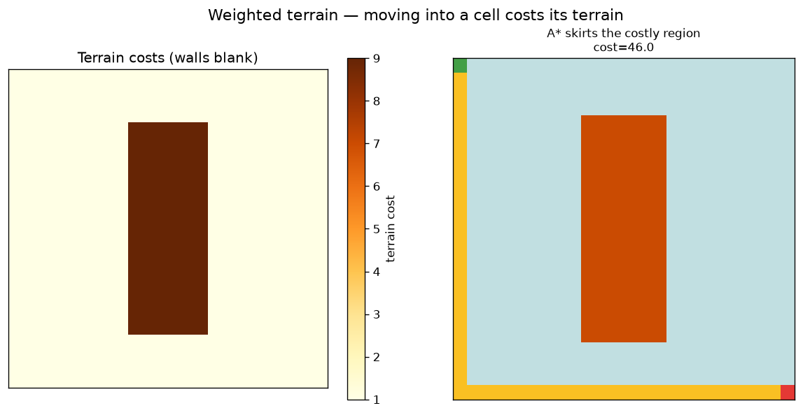
plot_costs — terrain heatmap

For weighted grids, plot_costs shows the terrain as a heatmap (walls left blank). plot_grid/animate_grid also shade the terrain underneath the search, so you can see what was explored over what terrain.

terrain = [[1.0]*24 for _ in range(24)]
for r in range(4, 20):
    for c in range(9, 15):
        terrain[r][c] = 9.0                      # an expensive plateau

r = gf.search_grid_costs(terrain, (0, 0), (23, 23), algorithm="astar", record=True)
gf.viz.plot_costs(terrain)                       # the heatmap
gf.viz.plot_grid(terrain, r)                     # A* skirting the costly region

Grid viz accepts either an ASCII map (digits 1–9 are costs) or the cost matrix you passed to search_grid_costs.

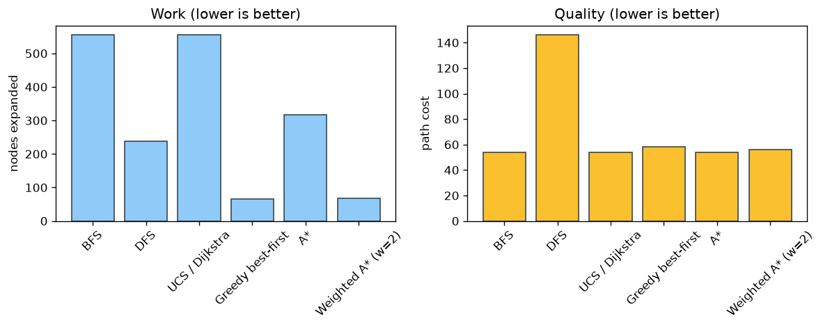
compare — work vs quality

Pass a dict {name: result}; get bar charts of nodes expanded (work) and path cost (quality).

results = {
    "BFS":    gf.search(maze, algorithm="bfs",    heuristic="zero"),
    "UCS":    gf.search(maze, algorithm="ucs",    heuristic="zero"),
    "Greedy": gf.search(maze, algorithm="greedy", heuristic="manhattan"),
    "A*":     gf.search(maze, algorithm="astar",  heuristic="manhattan"),
}
gf.viz.compare(results)

plot_frontier — the memory profile

Frontier size at each expansion step — the graph-search analogue of a convergence curve. Overlay several algorithms on one axis:

ax = None
for algo, h in [("bfs","zero"), ("ucs","zero"), ("astar","manhattan")]:
    r = gf.search(maze, algorithm=algo, heuristic=h, record=True)
    ax = gf.viz.plot_frontier(r, ax=ax, label=algo)

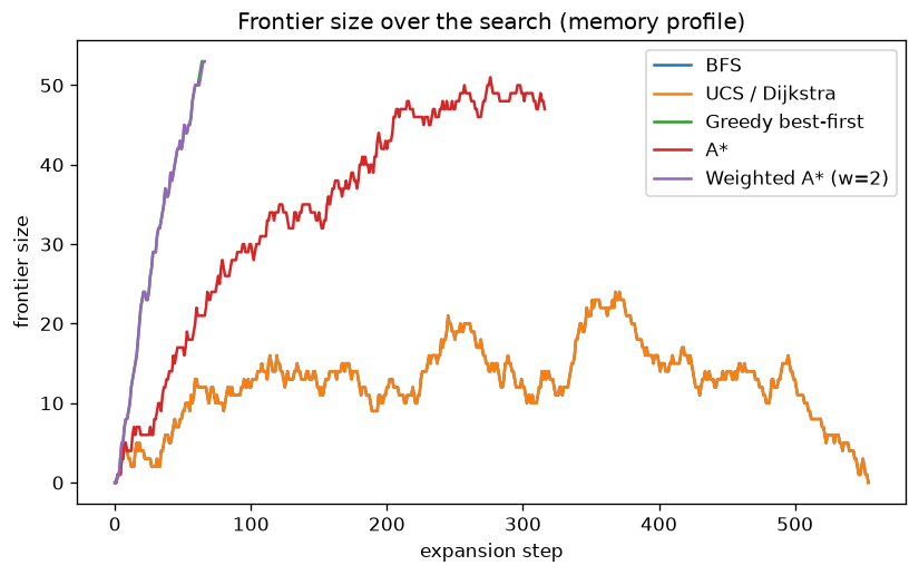
The flood algorithms grow a large frontier; informed ones keep it small.

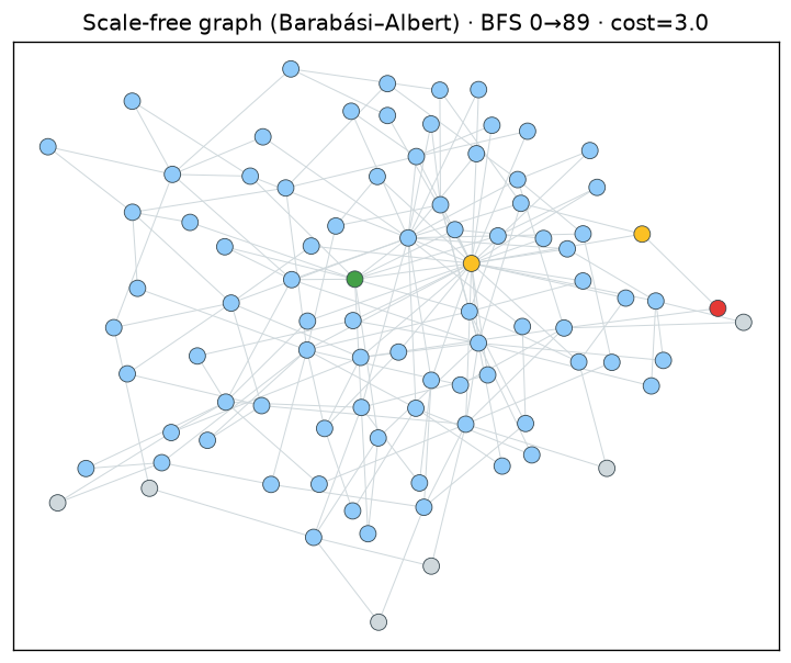
plot_graph — general graphs

Lay out an explicit graph and colour nodes by their role in the search (grey = untouched, blue = expanded, gold = path, green/red = start/goal). Uses a networkx spring layout if installed, else a circular layout.

edges = gf.gen_barabasi_albert(90, 2, seed=3)
r = gf.search_graph(90, edges, 0, 89, algorithm="bfs", record=True)
gf.viz.plot_graph(90, edges, r)

Reproduce these figures

Every image on this site is produced by one script:

python examples/build_docs_assets.py     # writes docs/assets/

See the API reference for each function's full signature.