Tutorial: comparing algorithms

The point of graphfinder is that the algorithms are the same loop — so comparing them is just a loop over names. This tutorial reproduces the headline figures.

Run every algorithm on one maze

import graphfinder as gf

maze = gf.random_maze_ascii(28, 28, 0.25, seed=2)

CONFIGS = [
    ("bfs", "zero"), ("dfs", "zero"), ("ucs", "zero"),
    ("greedy", "manhattan"), ("astar", "manhattan"),
    ("weighted_astar", "manhattan"),
]

for algo, h in CONFIGS:
    r = gf.search(maze, algorithm=algo, heuristic=h, record=True)
    print(f"{algo:16} cost={r.cost:6}  expanded={r.nodes_expanded:5}  "
          f"frontier={r.max_frontier_size}")

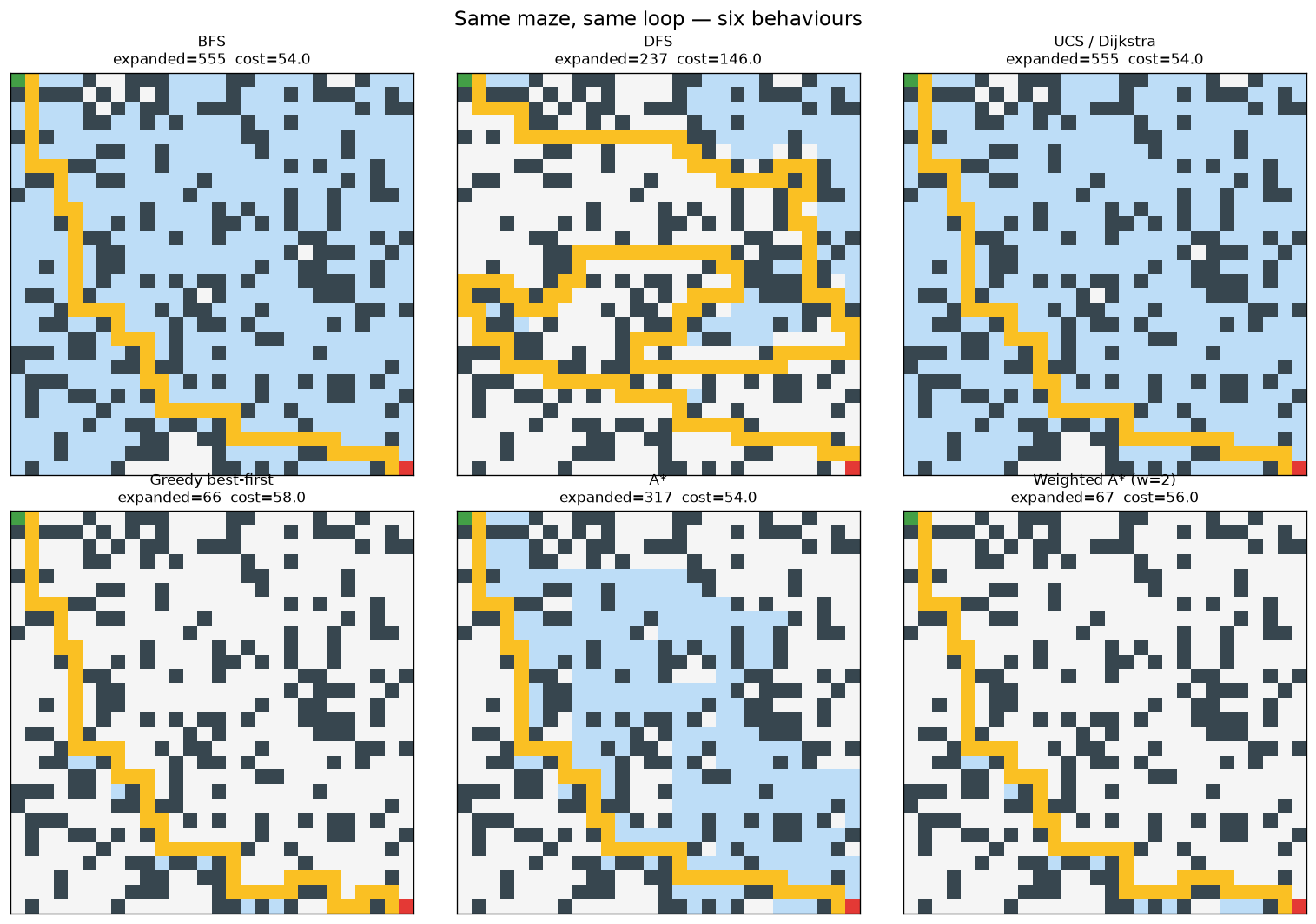
Typical output (same maze):

bfs              cost=  54.0  expanded=  555  frontier=...
dfs              cost= 146.0  expanded=  237  frontier=...
ucs              cost=  54.0  expanded=  555  frontier=...
greedy           cost=  58.0  expanded=   66  frontier=...
astar            cost=  54.0  expanded=  317  frontier=...
weighted_astar   cost=  56.0  expanded=   67  frontier=...

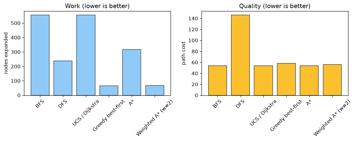
The story in one table: BFS/UCS are optimal but explore everything; DFS is cheap but its path is terrible; Greedy is cheapest to run but overshoots the optimum; A* is optimal and economical; Weighted A* gets near-optimal for almost Greedy-level work.

Visualize the trade-off

results = {name: gf.search(maze, algorithm=a, heuristic=h)
           for (a, h), name in zip(CONFIGS, ["BFS","DFS","UCS","Greedy","A*","WA*"])}
gf.viz.compare(results)

And the six explorations side by side:

import matplotlib.pyplot as plt
fig, axes = plt.subplots(2, 3, figsize=(13, 9))
for ax, (algo, h) in zip(axes.ravel(), CONFIGS):
    r = gf.search(maze, algorithm=algo, heuristic=h, record=True)
    gf.viz.plot_grid(maze, r, ax=ax)

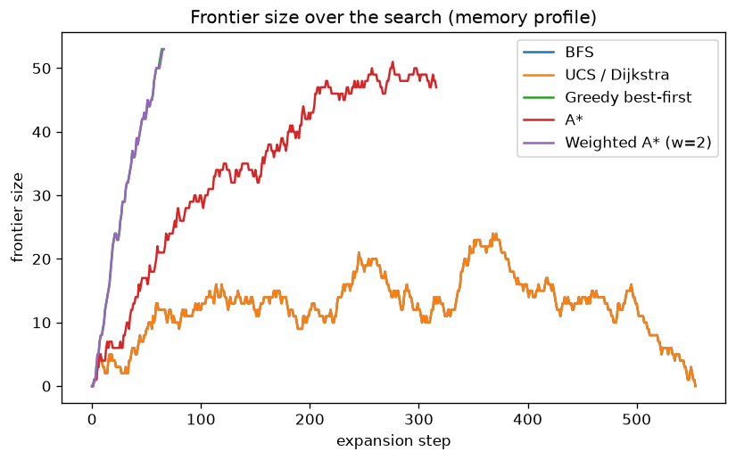
Memory profile

Frontier size over time separates the flood algorithms from the focused ones:

ax = None
for algo, h in [("bfs","zero"), ("ucs","zero"), ("greedy","manhattan"), ("astar","manhattan")]:
    r = gf.search(maze, algorithm=algo, heuristic=h, record=True)
    ax = gf.viz.plot_frontier(r, ax=ax, label=algo)

Bidirectional vs one-directional

bfs  = gf.search(maze, algorithm="bfs", heuristic="zero", record=True)
bidi = gf.search(maze, algorithm="bidirectional", record=True)
print(bfs.nodes_expanded, "vs", bidi.nodes_expanded)

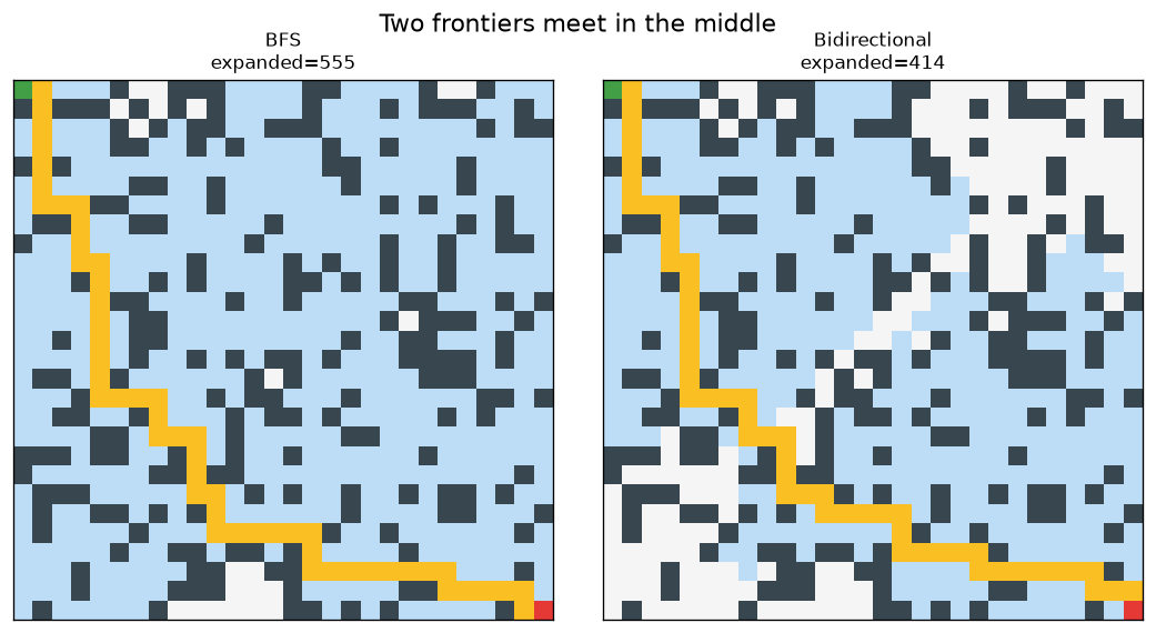
Two frontiers meeting in the middle expand far fewer nodes for the same optimal path.