Domains

A domain is the world you search over. graphfinder ships three, all behind the same Graph trait, so every algorithm works on every domain.

Grids / mazes

A rectangular lattice of cells, each free or a wall. Nodes are (row, col); orthogonal moves cost 1.0, diagonal moves (when enabled) cost √2. This is the canonical pathfinding teaching domain and the one the animations render.

maze = gf.sample_maze("wall")                      # built-in
maze = gf.random_maze_ascii(25, 25, 0.25, seed=0)  # reproducible random

r = gf.search(maze, algorithm="astar", heuristic="manhattan", diagonal=False)

ASCII format: # wall · S start · G goal · anything else free.

S.........
.####.###.
.#..#.#.#.
.#....#..G

The random generator does not guarantee solvability (so you can exercise the "no path" case) — check r.found.

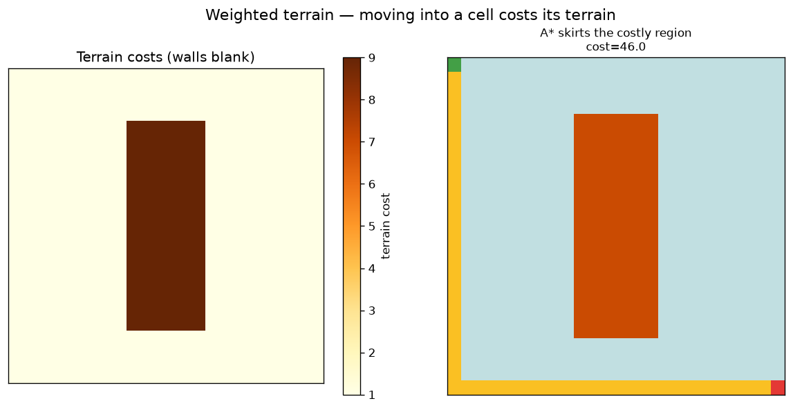
Weighted terrain

Cells are not just wall/free — every free cell has a terrain cost (default 1.0). Moving into a cell costs its terrain (× √2 for a diagonal step), so on a weighted grid Dijkstra/A* genuinely differ from BFS: the cheapest path is no longer the one with the fewest steps.

In an ASCII map, a digit 1–9 sets that cell's cost:

# Top row is expensive terrain (9); the bottom row is a cheap detour.
maze = "S99G\n1111"
gf.search(maze, algorithm="bfs").cost   # 19.0  — fewest steps, but expensive
gf.search(maze, algorithm="ucs").cost   # 5.0   — least cost, longer route

For arbitrary costs (beyond 1–9), pass a matrix to search_grid_costs; a cell that is ≤ 0 or non-finite is treated as a wall:

costs = [
    [1, 1, 1],
    [9, 0, 1],   # 0 ⇒ wall
    [1, 1, 1],
]
r = gf.search_grid_costs(costs, start=(0, 0), goal=(2, 0), algorithm="astar")

Visualize the terrain and how A* skirts the expensive region:

Heuristics on weighted grids

manhattan/euclidean/octile count grid steps, so they stay admissible only when every terrain cost ≥ 1 (the usual case). With sub-unit costs, use zero (→ Dijkstra) or a heuristic scaled by the minimum cost. See Heuristics.

Explicit weighted graphs

An adjacency structure held in memory (Compressed-Sparse-Row internally — cache-friendly, the standard layout for large graphs). Nodes are integers 0..n; you provide an edge list (u, v, weight).

edges = [(0, 1, 1.0), (1, 2, 2.0), (0, 2, 4.0)]
r = gf.search_graph(3, edges, start=0, goal=2, algorithm="dijkstra")
print(r.cost)   # 3.0  (0→1→2 beats the direct 0→2)

Random-graph generators

Reproducible (seeded) families, returned as edge lists ready for search_graph:

Generator	Models	Signature
gen_erdos_renyi(n, p, seed)	uniform random edges	G(n, p)
gen_barabasi_albert(n, m, seed)	scale-free / hubs	preferential attachment
gen_watts_strogatz(n, k, beta, seed)	small-world	rewired ring lattice

edges = gf.gen_barabasi_albert(90, 2, seed=3)
r = gf.search_graph(90, edges, 0, 89, algorithm="bfs", record=True)
gf.viz.plot_graph(90, edges, r)

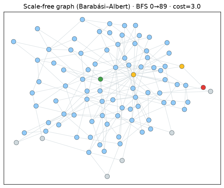
Nodes are coloured by their role in the search: grey = untouched, blue = expanded, gold = on the path, green/red = start/goal.

Implicit graphs (state spaces)

The graph that is never materialized — its successors are generated on demand. This is how classic puzzles are searched (you cannot store every state of a 15-puzzle), and where the Rust core's GIL-free expansion shines.

Provide a successor function; states are ints or tuples of ints:

# Word-ladder-style / arithmetic reachability
def successors(s):
    return [(s + 1, 1.0), (s * 2, 1.0)] if s < 1000 else []

r = gf.search(successors, start=1, goal=27, algorithm="bfs")

Because the state is an arbitrary tuple, you can encode puzzle boards, register machines, or any transition system. Pair it with a custom heuristic callable for A*/IDA*.

Writing a new domain (Rust)

A domain is one trait method — return each successor and its edge cost:

use graphfinder_core::Graph;

struct Knight;                  // a chessboard knight's moves
impl Graph for Knight {
    type Node = (i32, i32);
    fn neighbors(&self, &(r, c): &(i32, i32)) -> Vec<((i32, i32), f64)> {
        const D: [(i32, i32); 8] =
            [(1,2),(2,1),(-1,2),(-2,1),(1,-2),(2,-1),(-1,-2),(-2,-1)];
        D.iter().map(|(dr, dc)| ((r + dr, c + dc), 1.0)).collect()
    }
}

Every algorithm in the library now works on Knight unchanged. See Design & internals.